UmbrellaSampling
Table of Contents
About
Umbrella sampling is an advanced technique in Molecular Dynamics (MD) and Monte Carlo simulations used to calculate free energy profiles along a chosen reaction coordinate, especially in systems with high energy barriers. It overcomes sampling limitations by applying biasing potentials to different windows or regions along the reaction coordinate, allowing each window to sample effectively in that region.
Each biased simulation (or “window”) focuses on a specific part of the reaction coordinate, enabling the system to explore otherwise hard-to-reach configurations. Once data from all windows is collected, the biases are removed using reweighting techniques like the Weighted Histogram Analysis Method (WHAM). This yields an unbiased, continuous free energy profile, allowing for the study of rare events or transitions that standard MD simulations might not sample within feasible time scales.
In essence, umbrella sampling makes it possible to compute free energy landscapes and transition states by breaking down complex sampling tasks into manageable regions.
For more details find some literature on your own.
Preparing your system
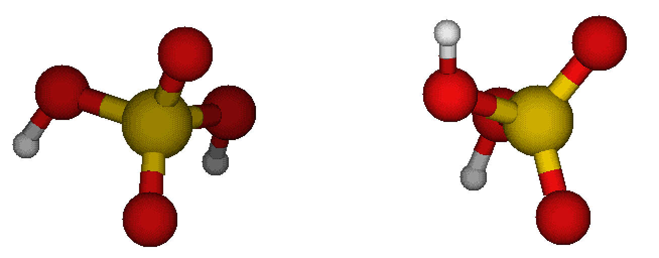
For this example, I will use two sulfuric acid molecules and try to get their free energy profile. I believe it is fair if you equilibrate the sulfuric acid (sa) molecules first:
JKMD 1sa.xyz -nf EQ_1sa -recenter -mb 300 -setvel 0 -langevin 0.01 -ns 10000 -dump 100 -par qany
Now we are ready for the contrained simulations
Constrained simulations
Now we will put the 2 molecules together and run MD at different distances from each other.
Let us first perform MD, where we place molecules in certain distance from each other, assing the harmonic potential to keep them in such a distance, perform equilibration, and run the representative MD simulation:
JKMD EQ_1sa/simcalc-LM.pkl -recenter -index -10 EQ_1sa/simcalc-LM.pkl -moveto [3.0--0.2--10,0,0] -harm 3.0--0.2--10 -langevin 0.01 -xtb GFN1-xTB -ns 100000 -dump 250 -follow -csvr 25 -ns 100000 -dump 250 -nf SA_SA_Langevin_CSVR -par q64,q48 -repeat 5
See that I am looping over the same numbers of harmonic potentials for the COM distance and the position of second molecule. Altough the molecules are equilibrated, they are not yet equilibrated in the presence of the external potential. Hence the equilibration where Langevin is used. For the real run, we recommend using canonical velocity rescaling (CSVR) thermostat as it does not have unphysical effect on the vibrations.
Hint
Storing structures durin equilibration is not as important. Storing structures during the actual run is important and perhaps is would be good to store not that well correlated structures, i.e. storing only every e.g. 50 ps. It is easy to generate massive amount of memory-heavy data here, so be careful.
Note
In the case, you have a cluster and a you place a molecules to some distance, there would be problems if the two overlap, so you can use the -moveto2 option to set some offset base on the cluster size. Like this they will not initially overlap and the molecule should get there during equilibration. See:
JKMD cluster.pkl -recenter molecules.pkl -moveto2 5.0 [0--0.2--10,0,0] ......
Note
For large molecules and ionic systems you will need to scan more than 10 Angstroms.
Analyzing the trajectory
Note
It is good to observe some features from the simulations and be sure that e.g. no evaporation occured nor something weird happened. For instance, check the max distance between atoms in each molecules. Those are store in the pickle file under the (log,maxA_distance) and (log,maxB_distance) columns.
For analysing the trajectory, use the JKumbrellaintegration command. You have to first enter to the SA_SA_Langevin_CSVR directory and run with suitable arguments:
cd SA_SA_Langevin_CSVR
JKumbrellaintegration -skip 100000 -symm
The -symm argument is used as we have two same molecules (factor of two in some equations) and -skip is used to skip the equilibration part of the trajectory. This will run for a bit but as it uses just 1 CPU, it can be performed on local computer. You can however submit it to the cluster if you used many repeats or used a long simulation:
sbatch -p qany --time 20:00 JKsend JKumbrellaintegration -skip 100000 -symm
Basically what happens is that first the histogram of COM distances is plotted along the evaporation coordinate
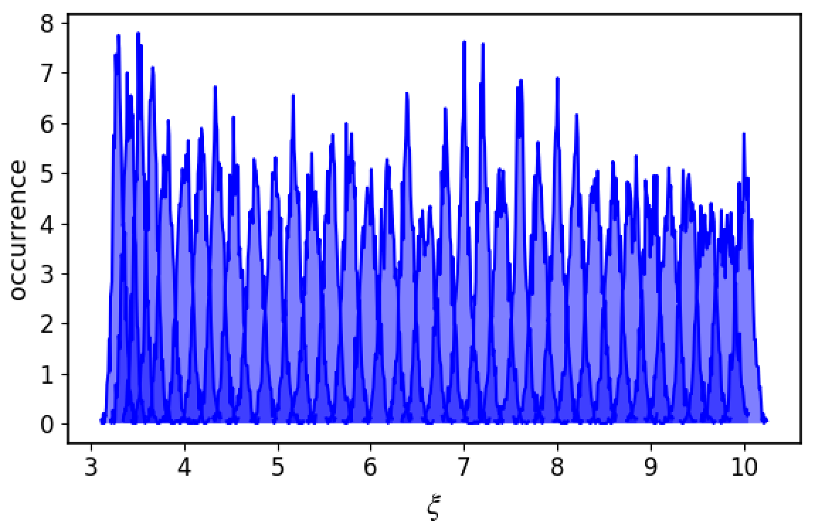
Note
Make sure the histograms from each window are partially overlapping with each other.
Then WHAM is used to obtain the free energy profile
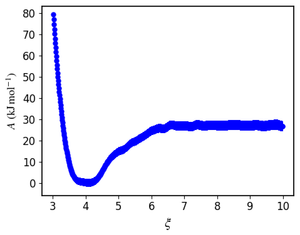
That one is further integrated over to give you the free energy binding of the SA-SA system. It is the last number in the umbrella_integration/output file. In this case we got -4.01 kcal/mol = -16.77 kJ/mol. As you can see the free energy depth is not exactly the same as the binding free energy!
Note
Make sure that the plotdG.png converges to a constant, otherwise there is something wrong with the simulation.
Citation
In this package, I use umbrella integration from github repository which you should cite: 10.5281/zenodo.164996. Also, you could cite Kaestner and Thiel (10.1063/1.2052648) whose equations are used in the umbrella integration. If you are using the uncertainties, then cite also 10.1063/1.2206775.